Using evotrees.jl for time series prediction
Introduction
In this post, I want to show an analysis of a time series that I’ve been working on. Usually, when dealing with time series, it is not so common to use machine learning algorithms (without at least trying more traditional models like the ARIMA family), but I still wanted to test how well a GBM model fits for these kinds of problems that are so popular.
NOTE: I don’t recommend starting with models of this type for time series problems. There are simpler models to understand that are less computationally expensive.
Dataset Preparation
Data Extraction
You can find the repository here, The codes you will see here, I prototyped in notebooks/tutorial.jl.
Now we start by making the corresponding imports.
using DataFrames
using Plots
using MLJ
using EvoTrees
using UrlDownload
using ZipFile
using HTTP
using CSV
using Dates
using Statistics
using MLJClusteringInterface
using Clustering
using FreqTables
using StatsPlots
using RollingFunctions
using StatsBase
using ShiftedArrays
There are several libraries in this section, and I must admit it took me some time to use each one. But anyway to start reading the dataframe, we can get it directly from its repository.
data_url = "https://archive.ics.uci.edu/ml/machine-learning-databases/00235/household_power_consumption.zip"
f = download(data_url)
z = ZipFile.Reader(f)
z_by_filename = Dict( f.name => f for f in z.files)
data = CSV.read(z_by_filename["household_power_consumption.txt"], DataFrame,)
The dataframe looks more or less like this:
     Row │ Date        Time      Global_active_power  Global_reactive_power  Voltage  Global_intensity  Sub_metering_1  Sub_metering_2  Sub_metering_3
         │ String15    Time      String7              String7                String7  String7           String7         String7         Float64?
─────────┼─────────────────────────────────────────────────────────────────────────────────────────────────────────────────────────────────────────────
       1 │ 16/12/2006  17:24:00  4.216                0.418                  234.840  18.400            0.000           1.000                     17.0
       2 │ 16/12/2006  17:25:00  5.360                0.436                  233.630  23.000            0.000           1.000                     16.0
       3 │ 16/12/2006  17:26:00  5.374                0.498                  233.290  23.000            0.000           2.000                     17.0
       4 │ 16/12/2006  17:27:00  5.388                0.502                  233.740  23.000            0.000           1.000                     17.0
       5 │ 16/12/2006  17:28:00  3.666                0.528                  235.680  15.800            0.000           1.000                     17.0
       6 │ 16/12/2006  17:29:00  3.520                0.522                  235.020  15.000            0.000           2.000                     17.0
       7 │ 16/12/2006  17:30:00  3.702                0.520                  235.090  15.800            0.000           1.000                     17.0
       8 │ 16/12/2006  17:31:00  3.700                0.520                  235.220  15.800            0.000           1.000                     17.0
       9 │ 16/12/2006  17:32:00  3.668                0.510                  233.990  15.800            0.000           1.000                     17.0
      10 │ 16/12/2006  17:33:00  3.662                0.510                  233.860  15.800            0.000           2.000                     16.0
      11 │ 16/12/2006  17:34:00  4.448                0.498                  232.860  19.600            0.000           1.000                     17.0
      12 │ 16/12/2006  17:35:00  5.412                0.470                  232.780  23.200            0.000           1.000                     17.0
      13 │ 16/12/2006  17:36:00  5.224                0.478                  232.990  22.400            0.000           1.000                     16.0
      14 │ 16/12/2006  17:37:00  5.268                0.398                  232.910  22.600            0.000           2.000                     17.0
    ⋮    │     ⋮          ⋮               ⋮                     ⋮               ⋮            ⋮                ⋮               ⋮               ⋮
 2075246 │ 26/11/2010  20:49:00  0.948                0.000                  238.160  4.000             0.000           1.000                      0.0
 2075247 │ 26/11/2010  20:50:00  1.198                0.128                  238.110  5.000             0.000           1.000                      0.0
 2075248 │ 26/11/2010  20:51:00  1.024                0.106                  238.840  4.200             0.000           1.000                      0.0
 2075249 │ 26/11/2010  20:52:00  0.946                0.000                  239.050  4.000             0.000           0.000                      0.0
 2075250 │ 26/11/2010  20:53:00  0.944                0.000                  238.720  4.000             0.000           0.000                      0.0
 2075251 │ 26/11/2010  20:54:00  0.946                0.000                  239.310  4.000             0.000           0.000                      0.0
 2075252 │ 26/11/2010  20:55:00  0.946                0.000                  239.740  4.000             0.000           0.000                      0.0
 2075253 │ 26/11/2010  20:56:00  0.942                0.000                  239.410  4.000             0.000           0.000                      0.0
 2075254 │ 26/11/2010  20:57:00  0.946                0.000                  240.330  4.000             0.000           0.000                      0.0
 2075255 │ 26/11/2010  20:58:00  0.946                0.000                  240.430  4.000             0.000           0.000                      0.0
 2075256 │ 26/11/2010  20:59:00  0.944                0.000                  240.000  4.000             0.000           0.000                      0.0
 2075257 │ 26/11/2010  21:00:00  0.938                0.000                  239.820  3.800             0.000           0.000                      0.0
 2075258 │ 26/11/2010  21:01:00  0.934                0.000                  239.700  3.800             0.000           0.000                      0.0
 2075259 │ 26/11/2010  21:02:00  0.932                0.000                  239.550  3.800             0.000           0.000                      0.0
                                                                                                                                   2075231 rows omitted
Dataset Cleaning
As can be seen, it is a quite large dataset and we can take the opportunity to create new variables, so we have the possibility to obtain relevant information.
#Create a variable
date_time = [DateTime(d, t) for (d,t) in zip(data[!,1], data[!,2])]

data[!,:date_time] = date_time

#Create variable for date
data[!,:year] = Dates.value.(Year.(data[!,1]))
data[!,:month] = Dates.value.(Month.(data[!,1]))
data[!,:day] = Dates.value.(Day.(data[!,1]))

#Create variable for time
data[!, :hour] = Dates.value.(Hour.(data[!,2]))
data[!, :minute] = Dates.value.(Minute.(data[!,2]))

#Create variable for weekends
data[!, :dayofweek] = [dayofweek(date) for date in data.Date]
data[!, :weekend] = [day in [6, 7] for day in data.dayofweek]
In addition, we notice that the variables are in String format. We can make some changes to put them in the appropriate form.
for i in 3:8
    data[!,i] = parse.(Float64, data[!,i])
end
data[!,1] = replace.(data[!,1], "/" => "-")
data[!,1] = Date.(data[!,1], "d-m-y")
Preliminary Visualizations
A classic way to plot all the variables is with the following code:
plot([plot(data[1:50000, :date_time],data[1:50000,col]; label = col, xrot=30) for col in ["Global_active_power", "Global_reactive_power", "Global_intensity", "Voltage", "Sub_metering_1", "Sub_metering_2", "Sub_metering_3"]]...)
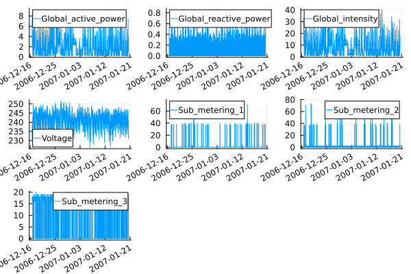
Note that we only take a sample of 50,000 data points to avoid overloading the graphs with information, and in the same way, we can create histograms.
plot([histogram(data[1:50000, col],label = col, bins = 20 ) for col in ["Global_active_power", "Global_reactive_power", "Global_intensity", "Voltage", "Sub_metering_1", "Sub_metering_2", "Sub_metering_3"]]...)

For now, we can recognize that the time series in its global variables have a white noise behavior, and Voltage also has it, however, it is the only one that seems to have a distribution that is similar to a normal distribution, while the sub-metering, are signs of use of household appliances.
A brief clustering with kmeans
In this section, we are interested in building a clustering model on the time series. The purpose? It is simply a way of evaluating behavior patterns over time, one hypothesis would be to see irregular behavior patterns over time, given that greater consumption would be seen at specific periods of the day or season.
An interesting issue that I was unaware of was that time series clustering is possible and you can use k-means, however in these cases, they cannot be treated from the same perspective, and other types of variants of these algorithms should be used to consider the temporality of neighboring observations when clustering. But since this project is just a toy, and the use of this technique is only for EDA, we will stick with the classical algorithm.
If you want to know more about this topic, yu can read this articule
Continuing with the problem, we can cluster by applying the following code.
X = data[!, 3:9]
transformer_instance = Standardizer()
transformer_model = machine(transformer_instance, X)
fit!(transformer_model)
X = MLJ.transform(transformer_model, X);
KMeans= @load KMeans pkg=Clustering
kmeans = KMeans(k=3)

mach = machine(kmeans, X) |> fit!

# cluster X into 3 clusters using K-means
Xsmall = MLJ.transform(mach);
selectrows(Xsmall, 1:4) |> pretty
yhat = MLJ.predict(mach)
data[!,:cluster] = yhat
In this case, we have 3 clusters that are ordered as follows.
cluster	nrow
CategoricalValue	Int64
1	1	741077
2	2	1257309
3	3	50894
And if we try to plot the clusters, we would have the following.
plot([scatter(data[1:20000, :date_time],data[1:20000,col]; group=data[1:20000,:].cluster, size=(1200, 1000), title = col, xrot=30) for col in ["Global_active_power", "Global_reactive_power", "Global_intensity", "Voltage", "Sub_metering_1", "Sub_metering_2", "Sub_metering_3"]]...)
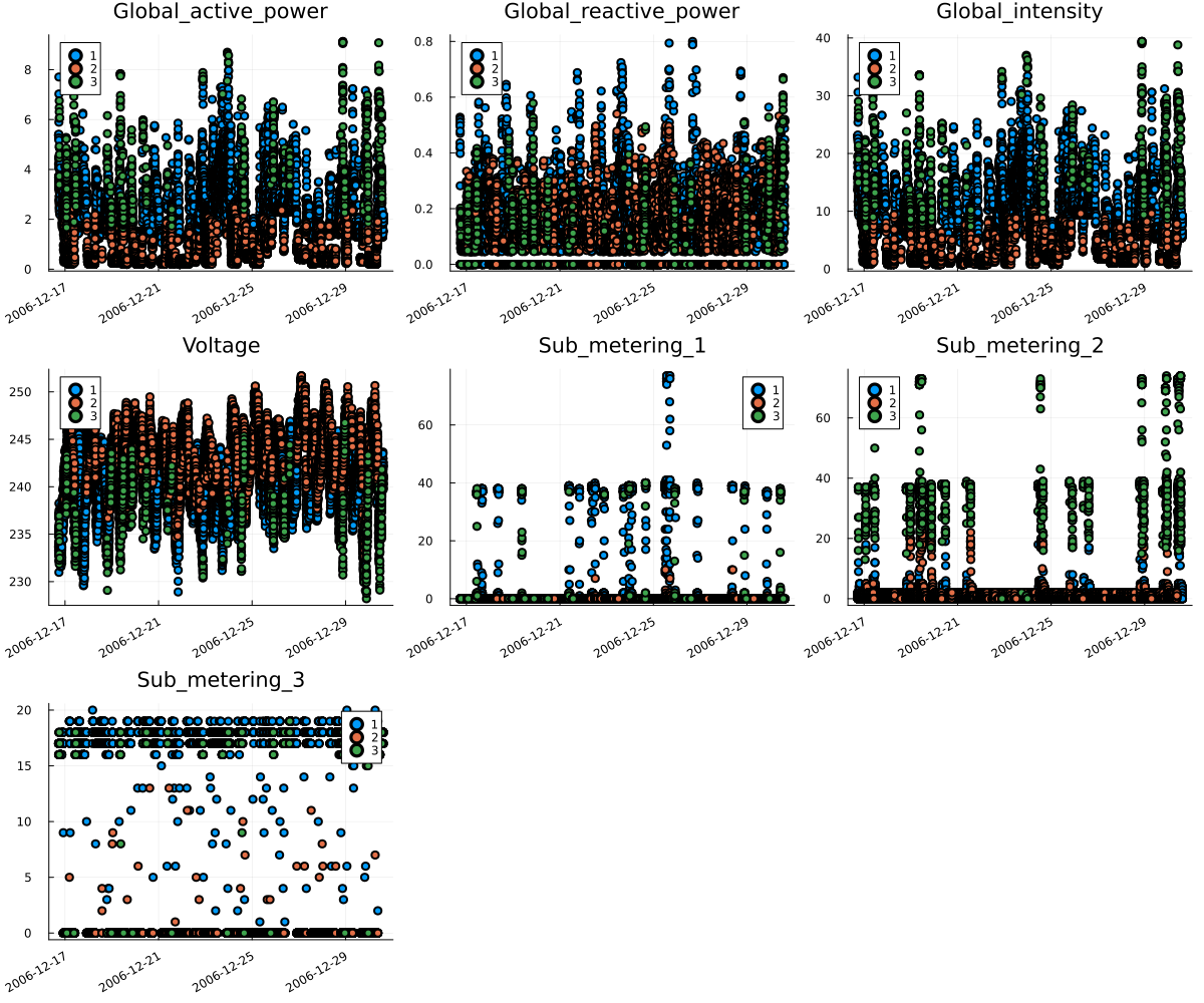
It looks a bit confusing, although if we look at the voltage variable, we can already size up a certain trend. For now, let’s consider a boxplot of the main variables but considering the clusters.
b1 =@df data boxplot(string.(:cluster), :Global_active_power, fillalpha=0.75, linewidth=2, title ="Global active power")
b2 =@df data boxplot(string.(:cluster), :Global_reactive_power, fillalpha=0.75, linewidth=2, title = "Global reactive power")
b3 = @df data boxplot(string.(:cluster), :Global_intensity, fillalpha=0.75, linewidth=2, title ="Global intensity")
b4 = @df data boxplot(string.(:cluster), :Voltage, fillalpha=0.75, linewidth=2, title = "Voltage")


plot(b1, b2, b3, b4 ,layout=(2,2), legend=false)
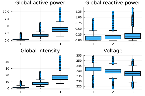
The truth is that we notice slight differences between the clusters, where we have certain consumption patterns in each category, but in some of their variables these do not necessarily lead us to any conclusion. However, as we had mentioned at the beginning, the idea of clustering was to study consumption patterns during time intervals, so we add the following.
h1 =heatmap(freqtable(data,:cluster,:dayofweek)./freqtable(data,:cluster), title = "day of week")
h2 =heatmap(freqtable(data,:cluster,:hour)./freqtable(data,:cluster), title = "hour")
h3 = heatmap(freqtable(data,:cluster,:month)./freqtable(data,:cluster), title = "month")
h4 = heatmap(freqtable(data,:cluster,:day)./freqtable(data,:cluster), title = "day")

plot(h1, h2, h3, h4 ,layout=(2,2), legend=false)

It might be a bit confusing initially, but let me take an example that might help you understand. If you take into account cluster 2, it corresponds to the lowest use of the global intensity used. If we go to the heatmap that represents the hours, we will see that the time where this pattern of behavior is most present is at night, which corresponds to the hours we are usually sleeping. I hope this make more sense.
This might give us a slight hint that time frames might be necessary, we’ll take this information for featuer engineering at this point later. Now let’s start with the next phase.
Using EvoTrees for prediction.
For now, we want to predict voltage. I’m not an expert in the field of electricity and consumption, but for a simple exercise, we will use the MLJ library (for Python users it would be equivalent to Scikit-Learn). Due to the amount of data and the algorithm we are going to use, it is not practical to perform training with cross-validation, this will take too much time, so we will prefer to only use a train/test split as a strategy.
let’s generate a lag and cut the data in the following way:
data[!, :lag_30] = Array(ShiftedArray(data.Voltage, 30))
replace!(data.lag_30, missing => 0);
And to assign the training and testing, we use the following.
train = copy(filter(x -> x.Date < Date(2010,10,01), data))
test = copy(filter(x -> x.Date >= Date(2010,10,01), data))
Then, we remove some variables that we won’t use to train the model, and we save our voltage variable.
select!(train, Not([:Date, :Time, :date_time, :cluster, ]))
select!(test, Not([:Date, :Time, :date_time, :cluster, ]))
y_train = copy(train[!,:Voltage])
y_test = copy(test[!,:Voltage])
Now we are going to apply a cyclical encoder to be able to work with the data, we have several new variables related to time (month, day, hour, among others), and all these variables will be more helpful if we allow extracting their cyclical character, that is why we use a trigonometric transformation
function cyclical_encoder(df::DataFrame, columns::Union{Array, Symbol}, max_val::Union{Array, Int} )
    for (column, max) in zip(columns, max_val)

        df[:, Symbol(string(column) * "_sin")] = sin.(2*pi*df[:, column]/max)
        df[:, Symbol(string(column) * "_cos")] = cos.(2*pi*df[:, column]/max)
    end
    return df
end
Finally, we can apply this new function to our dataset.
columns_selected = [:day, :year, :month, :hour, :minute, :dayofweek]
max_val = [31, 2010, 12, 23, 59, 7]
train_cyclical = cyclical_encoder(train, columns_selected, max_val)
test_cyclical = cyclical_encoder(test, columns_selected, max_val)
And finally, let’s train the model.
EvoTreeRegressor = @load EvoTreeRegressor pkg=EvoTrees verbosity=0
etr_start = EvoTreeRegressor(max_depth =15)

machreg = machine(etr_start, train_cyclical[!,14:end], y_train);
fit!(machreg);


pred_etr_train = MLJ.predict(machreg, train_cyclical[!,14:end]);
rms_score_train = rms(pred_etr_train, y_train)
println("The rms in train is $rms_score_train")

pred_etr = MLJ.predict(machreg, test_cyclical[!,14:end]);
rms_score = rms(pred_etr, y_test)
println("The rms in test is $rms_score")
This is our result:
- The rms in train is 2.5364451392238085
- The rms in test is 3.438565163838837
In this section, we plot the residual left by our model, and here we can detect some signs of overfitting, considering that our model has a much better score in the training dataset than in the test dataset. On the other hand, the plots are showing us that our model has biases in its predictions, it is not being able to recognize trends.

Finally, we can see how the predictions compare to the test data.
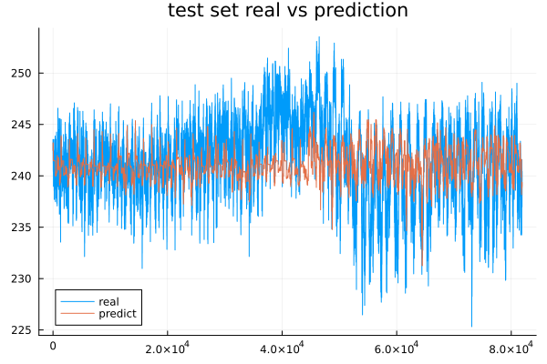
As we have confirmed earlier, the prediction does not seem to have been able to determine the magnitudes of the voltage in the testing of the dataset. Despite the fact that our variable is fairly stable over time, the model was trained with different parameters, but ultimately none of the options managed to show a significant improvement.
Conclusions
With this small exercise, we only tried to test that GBM, while a powerful tool and popular in places like Kaggle, requires a certain level of expertise both in the model and in the use case to achieve good performance. A naive approach may not generate results that satisfy the users. This, on one hand, requires:
- Understanding how to perform feature engineering for a time series, such as obtaining the decomposition of the time series. This can help capture trends that cannot always be obtained solely with the time horizon.
- Applying smoothing strategies like moving averages could help recognize the underlying pattern, but then you will need to estimate that moving average into the future.
Overall, time series analysis requires a deep understanding of the data, proper preprocessing techniques, feature engineering, and selecting appropriate models that can capture the specific patterns and dynamics of the data.